Don't trust small sample sizes
July 15, 2019We know that studies with small sample sizes have low power to detect effects. We also know that it's not always easy to get a big sample size. So a lot of studies are run with small sample sizes, and we probably miss some important effects because of low power. But small sample sizes can also cause the opposite problem, where we end up thinking effects are much bigger than they are.
To demonstrate, we'll use a simple setup where we simulate samples from two groups, control and treatment, and compare them with a t-test. This function generates two random samples, compares them, and returns the p-value for the t-test along with the standardized effect size (divided by the standard deviation):
simulate_t_test = function(control_mean, treatment_mean, sd, sample_size) {
    control_sample = rnorm(sample_size, control_mean, sd)
    treat_sample = rnorm(sample_size, treatment_mean, sd)

    est_control_sd = sd(control_sample)
    p_val = t.test(control_sample, treat_sample)$p.value
    est_effect = (mean(treat_sample) - mean(control_sample)) / est_control_sd

    tibble(est_effect, p_val)
}
We'll simulate these comparisons for a range of sample and effect sizes:
n_sim = 1000  # Number of samples to simulate
control_mean = 13.2
# Let's just assume the treatment and control have
#   the same standard deviation
control_sd = 5

study_table = tibble(sample_size = c(10, 20, 50, 100, 200),
                         effect_size = c(0, 0.1, 0.2, 0.5, 1.0)) %>%
    expand(sample_size, effect_size, sim_num = 1:n_sim) %>%
    mutate(treatment_mean = control_mean + (control_sd * effect_size))

sim_effects = study_table %>%
    rowwise() %>%
    do(sim_effect = simulate_t_test(control_mean, .$treatment_mean,
                                    control_sd, .$sample_size)) %>%
    unnest()
| sample size | effect size | sim | estimate | p |
|---|---|---|---|---|
| 10 | 0 | 1 | 0.39 | 0.37 |
| 10 | 0 | 2 | 0.18 | 0.71 |
| 10 | 0 | 3 | 0.92 | 0.09 |
| 10 | 0 | 4 | -0.48 | 0.23 |
| 10 | 0 | 5 | -0.63 | 0.34 |
| 10 | 0 | 6 | 1.06 | 0.05 |
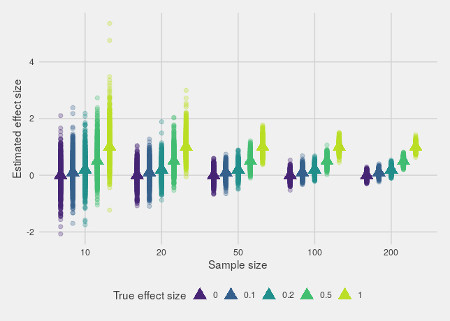
If we plot the estimated effects, we'll see what we expect: estimates from small sample sizes are much more variable than larger sample sizes, with a big spread around the true effect.
However, that's not actually the biggest issue. The real issue is that if there's any kind of bias towards only reporting significant effects (through p-hacking, publish or perish incentives or any other mechanism), the estimates found in smaller studies will be way off, either much too large or in the wrong direction entirely.
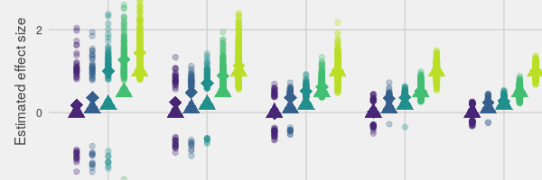
This can be seen most clearly if you only look at the estimates that are "significant":
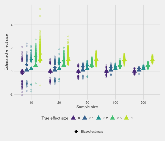
In fact, if the true effect size is small, then small studies can't provide an accurate estimate of the effect size while still being significant.
The probability of an estimate being in the wrong direction is called Type S error (wrong sign), while the amount that estimates exaggerate the true effect size is the Type M error (wrong magnitude). Both are discussed in this paper by Andrew Gelman and John Carlin.
R code for the plots
dodger = position_dodge(width = 0.8)
study_table %>%
    bind_cols(sim_effects) %>%
    ggplot(aes(x = factor(sample_size), colour = factor(effect_size),
               group = factor(effect_size))) +
    geom_point(aes(y = effect_size), size = 5, shape = 17, position = dodger) +
    geom_point(aes(y = est_effect), size = 2, alpha = 0.3, position = dodger) +
    scale_colour_viridis_d(begin = 0.1, end = 0.9) +
    labs(colour = "True effect size", y = "Estimated effect size",
         x = "Sample size") +
    theme_fivethirtyeight() +
    theme(legend.position = "bottom",
          axis.title = element_text())
study_table %>%
    bind_cols(sim_effects) %>%
    filter(p_val < 0.05) %>%
    group_by(sample_size, effect_size) %>%
    mutate(biased_est = mean(est_effect)) %>%
    ggplot(aes(x = factor(sample_size), colour = factor(effect_size), group = factor(effect_size))) +
    geom_point(aes(y = est_effect), size = 2, alpha = 0.3, position = dodger) +
    geom_point(aes(y = effect_size), size = 5, shape = 17, position = dodger) +
    geom_point(aes(y = biased_est, shape = "Biased estimate"),
               size = 5, position = dodger) +
    scale_colour_viridis_d(begin = 0.1, end = 0.9) +
    scale_shape_manual(values = c(18)) +
    guides(colour = guide_legend(override.aes = list(shape = 17))) +
    labs(colour = "True effect size", y = "Estimated effect size",
         x = "Sample size", shape = "") +
    theme_fivethirtyeight() +
    theme(legend.position = "bottom",
          axis.title = element_text())