P-values aren't trendy
July 10, 2019One of the worst phrases to come across when reading an academic article is "a trend towards significance", usually accompanied by a p-value somewhere in the 0.06 to 0.10 range. The implication is that we have some evidence "in the direction" of an effect, and if we had just collected a bit more data things would have kept moving in that direction until they finally crossed that p < 0.05 threshold.
The problem is that p-values don't move anywhere - the p-value you get out of your sample is a fixed quantity that was locked in as soon as you specified your design and collected your sample, and more importantly, set out your intentions for what you were going to test. If you go on to collect more data you're altering those intentions and destroying the whole framework that made your original p-value mean something.
To demonstrate why you can't infer any motion in either direction from a p-value, it's useful to look at what happens when there's no true effect and you perform statistical tests as each data point comes in.
Simulations
We'll simulate some data from 2 groups that both have exactly the same mean and variance. We'll generate 100 observations, and repeat the process 50 times.
library(tidyverse)

n_samples = 50
total_obs = 100

sim_data = tibble(sample_num = 1:n_samples) %>%
    expand(sample_num, obs = 1:total_obs) %>%
    mutate(sim_y1 = rnorm(n(), mean = 5.3, sd = 2),
           sim_y2 = rnorm(n(), mean = 5.3, sd = 2))
If we perform t-tests comparing the two means repeatedly, every time an observation comes in, we can generate almost 100 different p-values for each simulated dataset (it's not really worth testing the first 5 observations).
# T-test everything!
sim_data = sim_data %>%
  group_by(sample_num) %>%
  mutate(
    mean_y1 = cummean(sim_y1),
    mean_y2 = cummean(sim_y2),
    p_val = c(
      rep(NA, 5), # Skip the 1st 5 obs
      purrr::map_dbl(
        6:n(),
        ~ t.test(sim_y1[1:.x], sim_y2[1:.x])$p.value)
    )
  )
| sample_num | obs | sim_y1 | sim_y2 | mean_y1 | mean_y2 | p_val |
|---|---|---|---|---|---|---|
| 1 | 1 | 3.51 | 7.38 | 3.51 | 7.38 | NA |
| 1 | 2 | 7.55 | 5.16 | 5.53 | 6.27 | NA |
| 1 | 3 | 6.24 | 4.91 | 5.77 | 5.82 | NA |
| 1 | 4 | 3.70 | 5.05 | 5.25 | 5.62 | NA |
| 1 | 5 | 2.70 | 5.97 | 4.74 | 5.69 | NA |
| 1 | 6 | 8.40 | 3.65 | 5.35 | 5.35 | 1.00 |
| 1 | 7 | 7.05 | 5.15 | 5.59 | 5.32 | 0.78 |
| 1 | 8 | 5.06 | 6.21 | 5.53 | 5.44 | 0.92 |
| 1 | 9 | 4.11 | 9.24 | 5.37 | 5.86 | 0.58 |
| 1 | 10 | 3.36 | 4.44 | 5.17 | 5.72 | 0.51 |
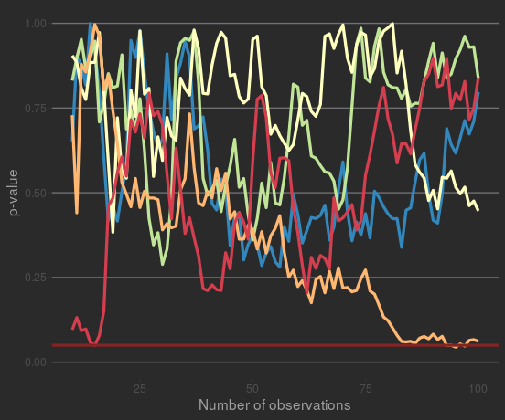
If we look at the p-values from a few of these simulated samples, it's clear they're all over the place. Some of them might move in one direction for multiple observations - but remember the data was specifically generated to have no true effect - they won't stay that way.
Some samples also test as 'significant' at some points, but they don't stay significant. Plotting the samples that test as 'significant' at least once:
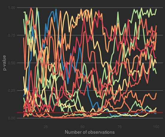
So a p-value that's close to significance (or even significant) isn't guaranteed to move towards significance. If at this point you're objecting to this demonstration, because these data were designed to have no effect... well, that's the whole point! p-values are supposed to show whether something's unlikely if there is no effect. A p-value of 0.06 could 'move' in any direction if you kept sampling.
Code for the plots
library(ggthemes)

to_plot = sample(1:n_samples, 5)

sim_data %>%
    filter(sample_num %in% to_plot, obs >= 10) %>%
    ggplot(aes(x = obs, y = p_val, group = sample_num, colour = rank(sample_num))) +
    geom_line(size = 1.2) +
    geom_hline(yintercept = 0.05, colour = scales::muted("red"),
               size = 1.2) +
    labs(x = "Number of observations",
         y = "p-value") +
    scale_y_continuous(limits = c(0, 1)) +
    scale_colour_distiller(palette = "Spectral") +
    guides(colour = 'none') +
    theme_hc(style = 'darkunica') +
    theme(axis.title = element_text())
sim_data %>%
    mutate(has_sig = any(p_val < 0.05)) %>%
    ungroup() %>%
    filter(has_sig, obs >= 10) %>%
    ggplot(aes(x = obs, y = p_val, group = sample_num, colour = rank(sample_num))) +
    geom_line(aes(colour = sample_num), size = 1.2) +
    geom_hline(yintercept = 0.05, colour = scales::muted("red"),
               size = 1.2) +
    labs(x = "Number of observations",
         y = "p-value") +
    scale_y_continuous(limits = c(0, 1)) +
    scale_colour_distiller(palette = "Spectral") +
    guides(colour = 'none') +
    theme_hc(style = 'darkunica') +
    theme(axis.title = element_text())